The Complete Guide to Polars for Data Science

Still Using Pandas? Here’s Why Polars Might Be Better.

Working with large datasets in Pandas can be frustrating. Slow performance, high memory usage, and long computation times make data processing inefficient. If you’ve hit these roadblocks, it’s time to explore Polars for Data Science, a lightning-fast DataFrame library built for speed and efficiency.

With parallel processing, lazy execution, and low memory usage, Polars handles millions of rows effortlessly. Whether you’re cleaning data, running analytics, or working with massive datasets, it can transform your workflow.

If you’re still using Pandas and want to master its full capabilities, check out our Pandas Complete tutorial for data science before making the switch.

This guide covers everything from loading and manipulating data to advanced optimizations. By the end, you’ll be ready to unlock Polars’ full potential in real-world data tasks.

1. Introduction to Polars

Polars is a high-performance DataFrame library built in Rust, designed for data scientists, analysts, and machine learning engineers working with large datasets. It offers faster performance and lower memory usage than Pandas, making it a powerful tool for data loading, preprocessing, and analysis.

Dataset & Code Repository

This guide uses the Customer Transactions & Spending Dataset (1M Rows), which includes customer demographics, spending behavior, and payment details. You can access the dataset and follow along with the exercises:

• Kaggle Dataset: Customer Transactions & Spending (1M Rows)
• GitHub Repository: Polars-Tutorial (Code)

To make learning easier, I’ve provided a Jupyter Notebook with all the code snippets. Clone the repo and try the exercises yourself.

2. Setup

Before using Polars, we need to ensure it’s installed in our environment. In this guide, I’m using Google Colab, where Polars may already be available. If it’s not, you can install it using:

!pip install polars

If you’re using a different environment like Jupyter Notebook or Anaconda, you may also need to install it. For detailed instructions, refer to the official Polars Installation Guide for setup instructions.

Importing Polars

import polars as pl

Setting Display Options

For better readability in Colab, configure Polars to display more rows and columns.

pl.Config.set_tbl_rows(10)  # Show 10 rows
pl.Config.set_tbl_cols(15)   # Show 15 columns
pl.Config.set_fmt_str_lengths(50)  # Increase max string column width

These settings make it easier to view large DataFrames without clutter.

3. Loading and Saving Data

Polars provides fast and memory-efficient methods for loading, saving, and streaming large datasets. It supports multiple file formats, including CSV, Parquet, JSON, IPC/Feather, and Avro, making it ideal for high-performance data processing. Parquet is often preferred for large datasets due to its efficient columnar storage and compression, which speeds up queries and reduces file size.

Reading CSV Files

CSV files are widely used for data storage and exchange. You can load a CSV file into Polars using:

# Read a CSV file
df = pl.read_csv("dataset/customer_spending_1M_2018_2025.csv")

# Display the first 5 rows
df.head(5)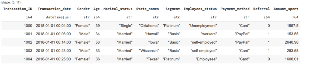

Reading Other File Formats

Polars supports multiple formats beyond CSV. You can read files using these methods:

# Read a Parquet file (Recommended for large datasets)
df_parquet = pl.read_parquet("dataset/online_store_data.parquet")

# Read a JSON file
df_json = pl.read_json("dataset/customer_data.json")

# Read an IPC/Feather file (Optimized for fast in-memory processing)
df_ipc = pl.read_ipc("dataset/online_store_data.feather")

# Read an Avro file (Commonly used for efficient data pipelines)
df_avro = pl.read_avro("dataset/online_store_data.avro")

Reading CSV with Additional Parameters

Polars allows customization when reading CSV files, making it easier to handle inconsistent datasets and optimize performance.

Skipping Rows

If a dataset contains metadata or unnecessary rows, you can skip specific rows while reading the file:

df = pl.read_csv(
    "dataset/customer_spending_1M_2018_2025.csv",
    skip_rows=2  # Skip first two rows if they contain metadata
)

Handling Headers in Raw Data

When working with datasets that lack proper headers, ensure the first row is interpreted correctly:

df = pl.read_csv(
    "content/customer_spending_1M_2018_2025.csv",
    has_header=True  # Ensures the first row is treated as headers
)

Reading CSV from a URL

Polars allows direct data loading from a URL, avoiding manual downloads.

df = pl.read_csv("https://example.com/data.csv")

Streaming Large Datasets

For large datasets, scan_csv() enables lazy loading, meaning only the required data is read instead of loading the entire dataset into memory.

Lazy Loading: A technique where data is loaded only when required, improving efficiency and reducing memory usage.

df_stream = pl.scan_csv("dataset/customer_spending_1M_2018_2025.csv")

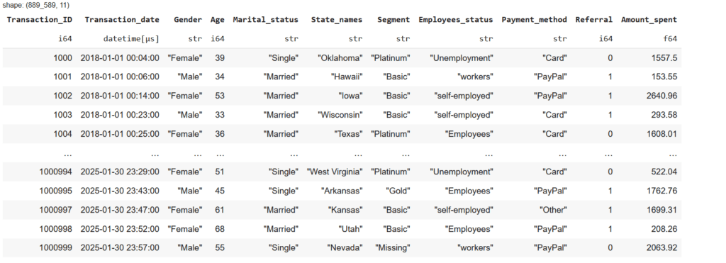
# Apply filtering before loading into memory
df_filtered = df_stream.filter(pl.col("Amount_spent") > 50)

# Collect to load the required data into memory
df_final = df_filtered.collect()
df_final.head(3)

The scan_csv() method is particularly useful when working with massive datasets that do not fit in memory. Instead of loading the entire file at once, it reads only the necessary data, significantly improving processing speed. By avoiding unnecessary data loading, it reduces memory consumption, making it ideal for big data analytics and preprocessing. For datasets larger than available RAM, scan_csv() ensures efficient data handling without crashes or slowdowns, enabling seamless analysis of large-scale data.

Saving Data Files

Polars allows saving DataFrames in multiple formats for efficient storage and sharing.

# Save DataFrame as CSV
df.write_csv("customer_data.csv")

# Save DataFrame as Parquet (recommended for large datasets)
df.write_parquet("customer_data.parquet")

# Save DataFrame as JSON
df.write_json("customer_data.json")

# Save DataFrame as IPC/Feather
df.write_ipc("customer_data.feather")

4. Data Exploration and Manipulation

After loading a dataset, the next step is to explore and manipulate it for meaningful analysis. This includes viewing the structure, selecting relevant data, filtering based on conditions, and sorting for better insights.

Polars provides high-performance operations for these tasks, making it faster than traditional libraries. Let’s go through some fundamental techniques.

Viewing Data (Head, Tail, Schema, Describe)

Before working on any dataset, it’s important to get a quick overview to understand its structure, column names, and data distribution.

Checking the First Few Rows

A quick way to check if the data was loaded correctly is by displaying the first few rows.

df.head()  # Shows the first 5 rows

This helps verify column names, data types, and potential inconsistencies in the dataset.

Viewing the Last Few Rows

To check if there are unexpected patterns or missing values at the end of the dataset, use:

df.tail()  # Shows the last 5 rows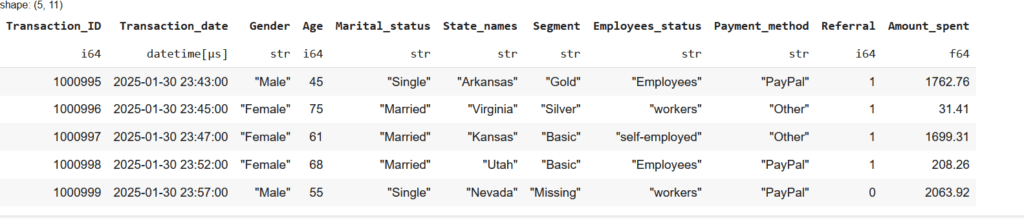

This is useful when working with log files, time-series data, or datasets where new entries are appended over time.

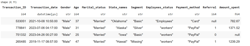
Retrieving Sample Rows from a DataFrame

To display a random sample of rows from a DataFrame, Polars provides the sample() function. This allows you to randomly select a specified number of rows, which is useful for quickly inspecting a dataset.

For example, to retrieve 4 random rows:

df.sample(n=4)

Checking the Structure of the Data

The .schema method gives a concise overview of column names and their data types, which is essential for understanding how data is stored.

df.schema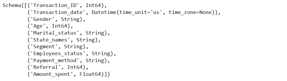

The output provides:

• Column names
• Data types (e.g., Int64, Float64, String, Boolean, etc.)

This helps in identifying incorrect data types, such as a date being stored as a string, which can lead to errors in analysis. It also ensures that numerical data is not mistakenly stored as text, preventing issues in calculations and comparisons. Additionally, understanding data types allows for better memory optimization by converting columns to more efficient formats, reducing overall resource usage.

Summarizing Data

For numerical columns, the describe() function provides a quick summary:

df.describe()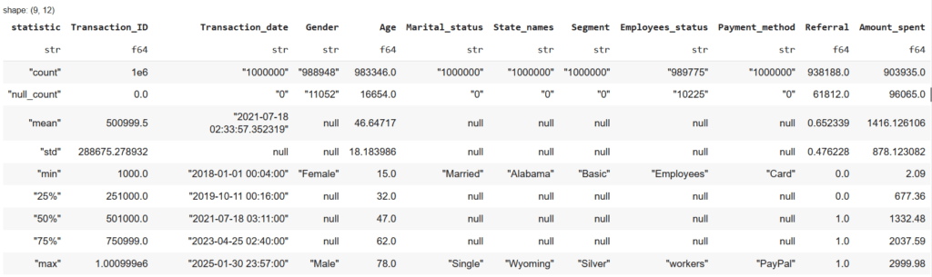

It displays:

• Count: Number of non-null values
• Mean: Average value
• Min & Max: Smallest and largest values
• Standard Deviation: How spread out the values are
• Percentiles (25%, 50%, 75%): Helps understand how data is distributed

Selecting, Filtering, and Slicing Data

Once we understand the dataset, we may need to focus on specific columns or rows.

Selecting Specific Columns

Sometimes, we don’t need all columns, so selecting only relevant ones improves performance.

Selecting One Column

df.select("Amount_spent")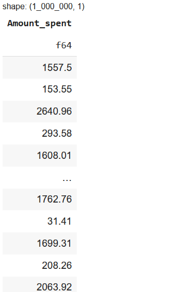

Selecting Multiple Columns

df.select(["Amount_spent", "Transaction_ID", "Gender"])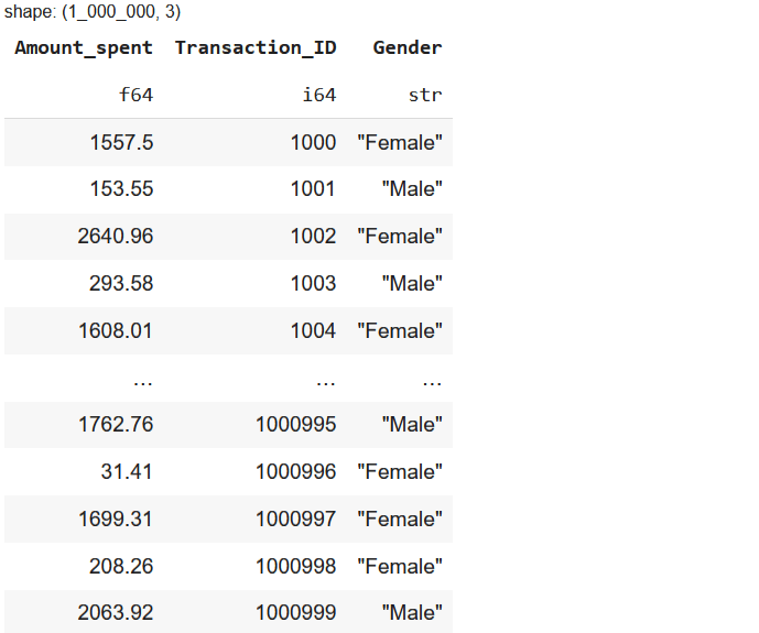

This reduces memory usage and makes further operations more efficient.

Filtering Rows Based on Conditions

Filtering helps in extracting only relevant rows from large datasets.

Filtering Rows Based on a Single Condition

To get transactions where Amount_spent is greater than $50:

df.filter(pl.col("Amount_spent") > 50)

Filtering Rows Based on Multiple Conditions

Similarly, you can filter for female customers who spent over $100 or married customers in California:

df.filter((pl.col("Amount_spent") > 100) & (pl.col("Gender") == "Female"))

df.filter((pl.col("Marital_status") == "Married") & (pl.col("State_names") == "California"))

Extracting a Specific Range of Rows (Slicing)

Slicing helps in retrieving specific portions of a dataset without loading everything into memory. This is useful when working with large datasets and needing only a subset of rows for quick analysis.

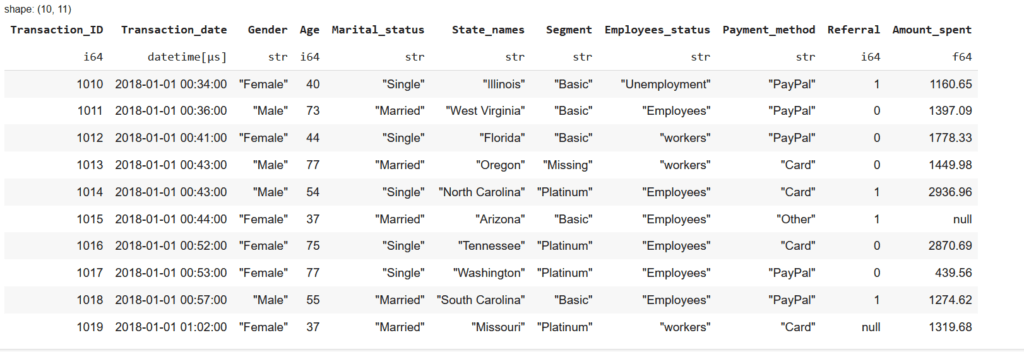
To extract rows 10 to 19 from the dataset:

Extract a Range of Rows by Index

df.slice(10, 10)  # Start at index 10, retrieve 10 rows (rows 10 to 19)

We can also slice the dataset for different use cases:

df.slice(0, 100)  # Retrieve the first 100 rows

df.tail(50)  # Get the last 50 rows

Slicing is especially useful for large datasets where loading everything into memory is not practical.

Sorting and Applying Conditions

Sorting helps in organizing data, finding top values, and ranking customers based on spending or activity.

Sorting Data in Ascending Order

df.sort("Amount_spent", nulls_last=True).head(4)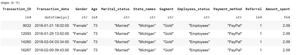

This arranges the dataset from lowest to highest spending.

Sorting Data in Descending Order

df.sort("Amount_spent", descending=True)

This sorts the dataset from highest to lowest, which is useful for:

• Identifying top spenders
• Finding the most frequently purchased items
• Ranking customers

Sorting by Multiple Columns

To sort first by Gender, then by Amount_spent (highest first):

df.sort(["Gender", "Amount_spent"], descending=[False, True], nulls_last=True).head(4)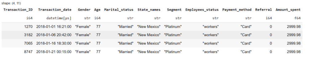

This sorts Gender alphabetically and then Amount_spent in descending order.

Applying Complex Conditional Queries

Instead of basic filters, we can combine multiple conditions.

Find Female Customers Who Spent More Than $100

df.filter((pl.col("Amount_spent") > 100) & (pl.col("Gender") == "Female"))

Get Customers Aged Between 25 and 40

df.filter((pl.col("Age") >= 25) & (pl.col("Age") <= 40))

These queries help segment the data for targeted analysis.

5. Data Cleaning and Preprocessing

Once we have explored the dataset, the next step is cleaning and preprocessing the data. This process involves handling missing values, converting data types, and manipulating text fields.

Inconsistent or messy data can cause errors in analysis and machine learning models, so it is crucial to clean and preprocess it properly.

Handling Missing Values

Missing values are common in datasets, often due to incomplete data collection, human error, or system failures. If not handled properly, they can skew results and cause issues in model training.

Checking for Missing Values

To check the number of missing values in each column:

df.null_count()

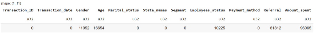
From this, we can see that Gender, Age, Employees_status, Referal and Amount_spent contain missing values.

Dropping Missing Values

If a column has a large number of missing values, it might be better to remove the entire column to avoid unreliable analysis. However, in our dataset, we do not have such a condition.

For example, if the Referral column had too many missing values, we could remove it like this:

df = df.drop("Referral")  # Removes the 'Referral' column
df.head(4)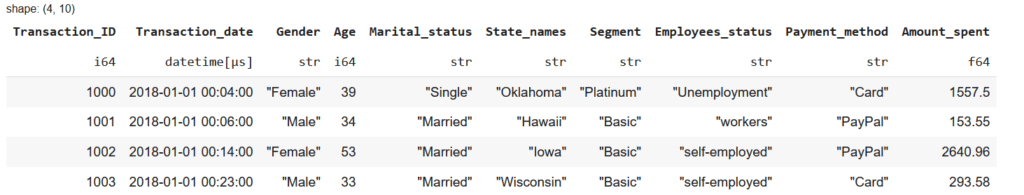

To drop rows with missing values in a specific column, use:

df.drop_nulls(subset=["Gender"])

This keeps only the rows where Gender is not null.

Filling Missing Values (Imputation)

Instead of dropping data, we can fill in missing values using different strategies:

Filling with a Fixed Value

If we want to replace missing values in Gender with "Unknown":

df = df.with_columns(pl.col("Gender").fill_null("Unknown"))

For numerical columns, we can replace missing values with zero or another fixed value:

df = df.with_columns(pl.col("Amount_spent").fill_null(0))

Filling with Statistical Measures

We can use mean, median, or mode to fill missing values based on existing data.

Replace missing values in Age with the median:

median_age = df["Age"].median()
df = df.with_columns(pl.col("Age").fill_null(median_age))

Replace missing values in Amount_spent with the mean:

mean_spent = df["Amount_spent"].mean()
df = df.with_columns(pl.col("Amount_spent").fill_null(mean_spent))

Replace missing values in Gender with the most frequent value (mode):

mode_gender = df["Gender"].mode()[0]  # Get most common value
df = df.with_columns(pl.col("Gender").fill_null(mode_gender))

Forward or Backward Filling

When dealing with time-series data, we can fill missing values based on previous or next values.

Forward fill (use the previous row’s value to fill the missing value):

df = df.with_columns(pl.col("Amount_spent").fill_null(strategy="forward"))

Backward fill (use the next row’s value to fill the missing value):

df = df.with_columns(pl.col("Amount_spent").fill_null(strategy="backward"))

This method is useful when data follows a logical sequence, such as stock prices or sales data.

Data Type Conversion

Sometimes, data is stored in the wrong format, causing issues when performing calculations or filtering.

Checking Data Types

df.schema

Optimizing Data Types

Polars automatically assigns appropriate data types when reading a dataset, as seen in our schema. While there are no incorrect types, converting certain columns can improve performance, memory efficiency, and data consistency.

Here are some useful transformations based on our dataset:

Convert Referral from Int64 to String (if it represents a category rather than a numerical value):

df = df.with_columns(pl.col("Referal").cast(pl.Utf8))  # Convert to String for better readability

Convert Age from Int64 to Float64 (if we need fractional values for calculations like average age):

df = df.with_columns(pl.col("Age").cast(pl.Float64))

Format Transaction_date to a standard YYYY-MM-DD format (useful if exporting data or for compatibility with other tools):

df = df.with_columns(pl.col("Transaction_date").dt.strftime("%Y-%m-%d"))

6. Advanced Data Transformations

Once our dataset is cleaned, the next step is to summarize, restructure, and extract insights for better analysis. Polars provides powerful transformation techniques that help in aggregating, reshaping, and analyzing trends.

Grouping and aggregations allow us to summarize data using statistical operations, such as calculating totals, averages, and counts. Pivoting and melting help reshape data for better representation, making it easier to analyze different categories. Rolling and expanding windows are useful for time-series analysis, enabling us to calculate trends over a specific period.

These transformations are essential for business analytics, forecasting, and reporting, allowing us to derive meaningful insights from raw data.

GroupBy and Aggregations

Grouping data is essential for analyzing trends, summarizing sales, and calculating metrics across different categories.

Grouping data means splitting it into subsets based on a categorical column and then applying an aggregation function (sum, mean, count, etc.) to each group.

For example:

• Finding total revenue per region
• Calculating average order value per customer
• Counting number of purchases per product category

To calculate total spending per gender:

df.group_by("Gender").agg(pl.sum("Amount_spent"))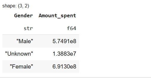

To calculate total amount spent by Gender and Payment Method:

df.group_by(["Gender", "Payment_method"]) \
  .agg(pl.sum("Amount_spent").cast(pl.Int64)) \
  .sort(["Gender", "Payment_method"])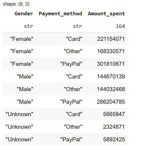

Grouping by multiple columns helps in multi-dimensional analysis.

Common aggregation functions include:

To calculate multiple statistics:

df.group_by("Gender").agg([
    pl.sum("Amount_spent").alias("Total Spent"),
    pl.mean("Age").alias("Average Age"),
    pl.len().alias("Customer Count")
])

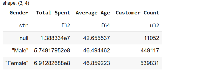
This summarizes spending, average age, and customer count per gender.

Pivoting DataFrames

Pivoting helps reshape data from a long format to a wide format, where unique values in one column become separate columns. This makes analysis easier by structuring aggregated values clearly, which is useful in business intelligence and reporting.

For example, to see total spending by each Gender for different Payment Methods, we can pivot the data so that each Payment Method becomes its own column:

df.pivot(
    values="Amount_spent", 
    index="Gender", 
    columns="Payment_method", 
    aggregate_function="sum"
)

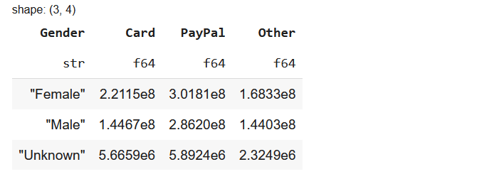
This transformation ensures that instead of repeating Payment Methods across rows, they are structured as separate columns, making it easier to analyze spending patterns. Pivoting is commonly used when working with summarized data that needs to be displayed in a more structured way.

7. Performance Optimization Techniques

Polars is designed for speed and efficiency, making it a great alternative to Pandas when working with large datasets. It optimizes performance by reducing memory usage and leveraging multi-threading, allowing faster execution even with millions of rows.

One key advantage is lazy execution, where computations are delayed until needed. This avoids unnecessary operations and improves efficiency. Polars also manages memory effectively by using optimized data types, reducing storage requirements without sacrificing accuracy. Additionally, it takes advantage of multi-threaded processing, distributing tasks across multiple CPU cores to handle computations faster.

These optimizations make Polars a powerful choice for data analysis, machine learning, and large-scale processing.

Lazy Execution for Speed and Efficiency

Lazy execution is one of Polars’ key optimizations that helps improve performance. Instead of executing each operation immediately, Polars builds an optimized execution plan and evaluates everything at once. This approach avoids unnecessary calculations, ensuring that only the required queries are executed when needed. As a result, memory usage is reduced, processing speed is improved, and large datasets can be handled more efficiently without loading everything into memory.

Using LazyFrames for Efficient Execution

Lazy execution is applied by using scan_csv() instead of read_csv(), which loads data only when required:

df_lazy = pl.scan_csv("dataset/large_customer_data.csv")

At this stage, no data is loaded into memory. Instead, df_lazy stores a query plan. To execute the query and retrieve only the necessary data, we use .collect():

df_final = df_lazy.filter(pl.col("Amount_spent") > 100).collect()

This method ensures that only the filtered data is loaded into memory, making it much more efficient for handling large datasets. Lazy execution is particularly useful for big data processing, ETL pipelines, and performance-critical applications, where avoiding unnecessary computations can significantly speed up workflows.

Memory Management (Efficient Data Types)

Optimizing memory usage is essential when handling large datasets. Using efficient data types helps reduce memory consumption without compromising precision. Choosing the right types can significantly improve performance, especially when working with millions of rows.

For example, smaller numerical types consume less memory:

• float32 instead of float64 reduces memory usage by half while maintaining sufficient precision.
• int32 instead of int64 minimizes storage for integer values.
• Converting text-based columns (object) to categorical types stores unique values more efficiently.

Converting Data Types for Optimization

To optimize memory usage, we can explicitly define data types when loading a dataset:

df = pl.read_csv(
    "dataset/customer_spending_1M_2018_2025.csv",
    schema_overrides={"Transaction_ID": pl.Int32, "Amount_spent": pl.Float32}
)

By specifying schema overrides, we ensure that large numerical values don’t take up unnecessary space while still maintaining accuracy.

To check how much memory a DataFrame consumes:

df.estimated_size()

This provides insights into the dataset’s memory footprint, helping us fine-tune data types for better efficiency.

Multi-threaded Processing

Polars is built to take full advantage of multi-threaded processing, making it significantly faster than Pandas, which primarily operates in a single-threaded mode. By default, Polars automatically optimizes performance by distributing computations across multiple CPU cores, ensuring faster execution for large datasets.

Unlike traditional data processing tools, Polars does not require manual multi-threading setup—it efficiently handles parallel computations in filtering, aggregations, and complex queries. This makes it ideal for big data analytics, large-scale computations, and performance-critical applications.

Parallel Processing in Aggregations

Polars automatically utilizes multiple threads when performing operations like filtering and grouping. For example, when calculating total spending per gender, the computation is distributed across available CPU cores:

df.group_by("Gender").agg(pl.sum("Amount_spent"))

Even without explicitly setting up parallelization, Polars ensures that grouping and aggregations run efficiently.

For advanced control, we can manually adjust the number of rows processed in parallel:

pl.Config.set_tbl_rows(4)  # Adjusts how many rows are processed in parallel

By combining lazy execution with multi-threaded processing, Polars significantly outperforms Pandas in handling large datasets, making it a powerful choice for high-performance data analysis.

8. SQL-like Queries with Polars

Polars allows users to run SQL-style queries directly on DataFrames, making it a powerful option for those familiar with SQL. This feature enables seamless integration between SQL and Python, allowing database professionals to work efficiently without switching to DataFrame operations. It also improves query readability, as SQL syntax can often be more intuitive for complex filtering, grouping, and aggregations. By combining SQL queries with Polars’ high-performance execution, users can analyze large datasets more efficiently while leveraging familiar query patterns.

Running SQL Queries in Polars

We can execute SQL queries directly on a Polars DataFrame using the built-in sql_context() method.

from polars import SQLContext  

sql_context = SQLContext()

# Register DataFrame as a SQL table
sql_context.register("customers", df)

# Run SQL query
result = sql_context.execute("SELECT Gender, SUM(Amount_spent) FROM customers GROUP BY Gender")

# Convert to Polars DataFrame
df_result = result.collect()
print(df_result)

This query retrieves total spending per gender, just like in a traditional SQL database.

Filtering and Aggregation with SQL Queries

Polars SQL can also be used for more complex operations, such as filtering and multiple aggregations:

result = sql_context.execute("""
    SELECT Gender, Payment_method, COUNT(*) AS Total_Transactions, AVG(Amount_spent) AS Avg_Spent
    FROM customers
    WHERE Amount_spent > 50
    GROUP BY Gender, Payment_method
    ORDER BY Avg_Spent DESC
""").collect()

print(result)

Other SQL Operations in Polars

Beyond simple filtering and aggregation, Polars supports a range of SQL-based operations to manipulate and analyze data efficiently. Here are some examples of what you can do:

• Joining Tables: Combine multiple datasets using INNER JOIN, LEFT JOIN, or RIGHT JOIN to merge customer transactions with additional details.
• Subqueries: Use nested SQL queries to filter data based on computed results, such as selecting customers with above-average spending.
• Window Functions: Apply ranking, cumulative sums, or moving averages over partitions of data, useful for time-series analysis.
• Conditional Expressions: Use CASE WHEN for creating new categories or handling missing values dynamically.
• String Operations: Perform text transformations like LOWER(), TRIM(), and CONCAT() directly in SQL.
• Date and Time Processing: Extract YEAR(), MONTH(), or calculate differences using DATEDIFF().
• Sorting and Limiting: Order query results and retrieve the top N rows with ORDER BY and LIMIT.

SQL queries in Polars provide flexibility, speed, and scalability, making it easy to integrate traditional database-style querying within Python workflows. Whether working with large-scale analytics, structured reporting, or complex joins, Polars’ SQL engine delivers familiar syntax with high-performance execution.

9. Final Thoughts

Polars for Data Science is transforming how we handle large-scale data processing in Python. With its Rust-powered performance, lazy execution, and multi-threaded capabilities, it offers a significant advantage over Pandas when working with massive datasets.

If you’re dealing with big data, performance bottlenecks, or memory constraints, Polars for Data Science is a superior choice that ensures efficiency without sacrificing usability.

When Should You Use Polars?

• For large datasets that exceed RAM, where Pandas struggles
• For performance-critical tasks, including ETL pipelines and analytics
• For memory-efficient workflows, reducing overhead in cloud environments
• For SQL-style querying, providing a smooth transition for database users
• For complex data transformations, including aggregations and filtering

That said, Pandas still has its place, especially for smaller datasets, seamless integration with libraries like Scikit-learn, and quick exploratory analysis. However, for serious data science, analytics, and machine learning workflows, Polars is the future-ready alternative you should explore.

What’s your experience with Polars? If you’ve used it, I’d love to hear your thoughts, drop a comment below!

10. Resources & Further Learning

• Polars Official Documentation – The best place to start learning the framework.
• Polars GitHub Repository – Stay updated with the latest developments.
• Kaggle Datasets & Polars Notebooks – Hands-on practice with real datasets.
• Polars Discussions on Stack Overflow – Troubleshooting and community Q&A.