Mastering NLP: A Journey Through Sentiment Analysis

Decoding Sentiments with Python: An NLP Journey from Novice to Expert

Mastering NLP: A Journey Through Sentiment Analysis — From Novice to Expert with Python. (Image: AI-generated)

Natural Language Processing (NLP) stands at the exciting intersection of artificial intelligence and human communication, enabling machines to understand and respond to us in remarkably human ways.

NLP enhances search functionalities and powers conversational agents, revolutionizing our interaction with technology. This article provides a clear and engaging exploration of the fundamentals of NLP and its applications in the real world. It’s designed for professionals, data science enthusiasts, and newcomers alike. Join us as we delve into the capabilities of NLP, making this advanced technology accessible to everyone.

In this article, we’re going on a fun and informative journey into Natural Language Processing (NLP), aiming to:

• Clarify NLP: Introduce you to the fundamentals of NLP, making it easy to grasp.
• Highlight Use Cases: Discuss various NLP applications to demonstrate its versatility.
• Detail Text Preprocessing: Walk through the essential steps of preparing text for analysis.
• Implement Machine Learning: Apply machine learning techniques in the context of sentiment analysis, from model training to evaluation.

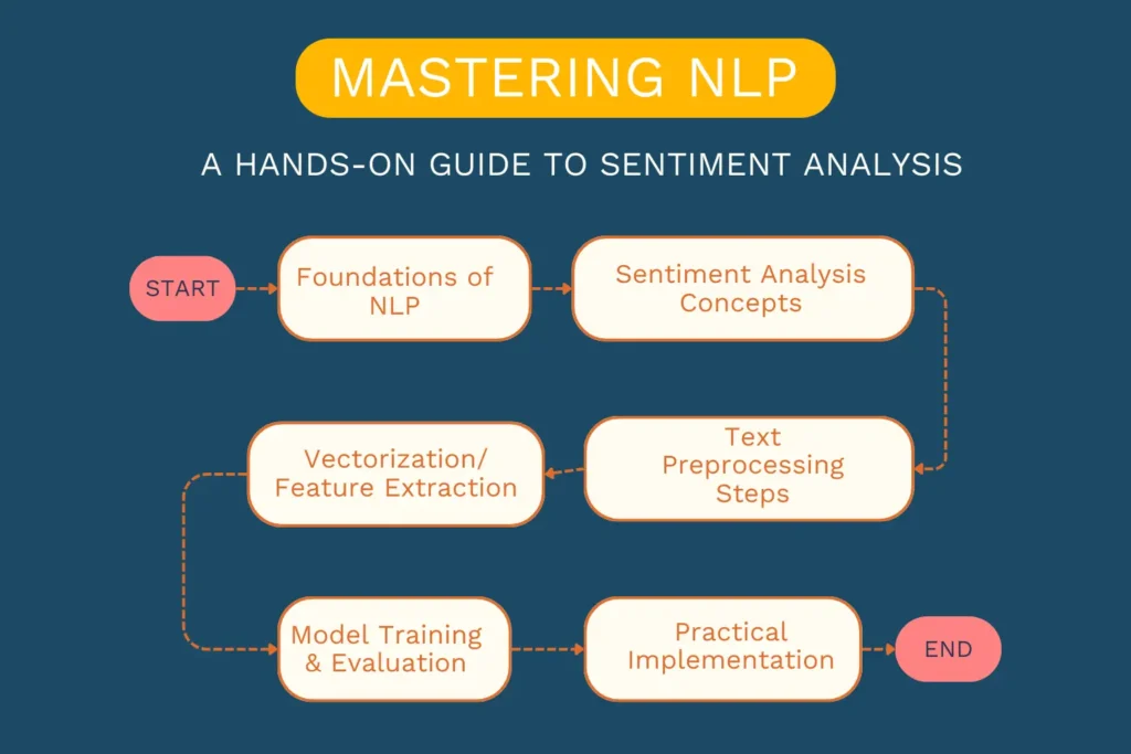
By the end of this journey, you’ll not only grasp the basics of NLP but also learn how to apply it in sentiment analysis, highlighting its vast potential. Let’s dive into the exciting world of NLP. First, here’s a quick overview of the topics we’re going to explore.

Table of contents

1. Foundations of Natural Language Processing

2. The Process of Sentiment Analysis

3. Text Preprocessing Techniques

4. Machine Learning for Sentiment Analysis

5. Conclusion: Unlocking Insights Through Sentiment Analysis

6. Wrapping up

7. Reference and Further reading

1. Foundations of Natural Language Processing

1.1 What is NLP?

NLP is the art of teaching computers to understand and respond to human language, creating a bridge between human thought and computer understanding.

At its core, Natural Language Processing, or NLP, is a technology that allows computers to understand, interpret, and respond to human languages in a way that is both meaningful and useful. Think of it as teaching computers to comprehend our words just as we do, bridging the gap between human communication and digital data processing.

Looking for a beginner-friendly introduction to AI?
Explore the Fundamentals of AI to understand what AI is, how it works, and why it’s transforming the way we live and work.

1.2 Why is NLP Important?

NLP stands as a cornerstone in the realm of artificial intelligence, significantly impacting how we interact with technology. It powers search engines, enables voice-operated gadgets, and manages customer service chatbots, making our digital experiences more intuitive and natural. By processing and analyzing vast amounts of natural language data, NLP helps in extracting insights, making decisions, and improving human-machine interactions.

1.3 NLP Use Cases

Natural Language Processing (NLP) finds its application across a wide spectrum of technologies, enhancing our ability to communicate with machines and process vast amounts of textual data efficiently. From simplifying user interactions to extracting valuable information from unstructured data, NLP’s versatility is showcased in several key areas.

• Sentiment Analysis: Identifies emotions in text, classifying them as positive, negative, or neutral.
• Named Entity Recognition (NER): Identify names, places, and other specific information from texts.
• Text Summarization: Create short, coherent summaries of longer documents.
• Question Answering: Answer user queries with information extracted from a given dataset.
• Machine Translation: Automatically translate text from one language to another.
• Chatbots: Engage in human-like conversations to provide customer support or information.
• Speech Recognition: Convert spoken language into text for further processing or action.
• Content Recommendation: Suggest relevant articles, movies, or products based on user preferences and history.
• Spell Checking and Grammar Correction: Identify and correct spelling and grammatical errors in texts.
• Search Optimization: Improve the relevance of search engine results based on the natural language query context.

Having explored the many uses of NLP, we’re now going to focus on something special: Sentiment Analysis. This lets us find out what people really think and feel based on what they write.

Next, we’ll dive into Sentiment Analysis, showing you step by step how it works and how you can use it too. This part of our article is all about making Sentiment Analysis clear and easy for everyone, no matter if you’re just starting out or already know a bit about NLP. Let’s get started and see how Sentiment Analysis helps us understand people’s emotions through text.

2. The Process of Sentiment Analysis

In this section, we shift our focus to Sentiment Analysis, illustrating its role as a cornerstone example to navigate through various NLP concepts. This involves text preprocessing, analyzing sentiments, and fitting data into machine learning models, offering us a lens to view how machines interpret human emotions and opinions expressed in text.

2.1 Understanding Sentiment Analysis

Sentiment Analysis, at its core, is the computational study of people’s opinions, feelings, evaluations, attitudes, and emotions expressed in written text. It involves analyzing text data to determine the sentiment behind it, categorizing it as positive, negative, or neutral. This technique is widely used to gauge consumer sentiment, monitor brand reputation, and understand customer experiences.

2.2 Potential Applications and Benefits in Various Industries

The versatility of sentiment analysis extends across multiple domains, demonstrating its capacity to provide actionable insights:

• Marketing and Brand Management: Companies can monitor social media sentiment about their brand or products, tailoring marketing strategies to address public perception.
• Finance and Market Research: Analyzing news articles, social media buzz, and financial reports through sentiment analysis helps predict market trends and investor sentiments, guiding investment strategies.
• Customer Service: Feedback and reviews undergo sentiment analysis to highlight areas of customer satisfaction or discontent, enabling businesses to refine their services or products.
• Healthcare: Patient feedback and online discussions can be analyzed to improve healthcare services, patient engagement, and treatment outcomes.

By harnessing sentiment analysis, industries gain a deeper understanding of the public’s opinions and emotions, leading to improved strategies, services, and products tailored to meet their audience’s needs.

Now that we’ve established what Sentiment Analysis is and its significance, let’s move into the practical application. We’ll be using a specific dataset to illustrate how sentiment analysis can be implemented effectively.

2.3 Working with the IMDB Movie Reviews Dataset

For our hands-on exploration, we’ve chosen the IMDB Dataset of 50K Movie Reviews from Kaggle. This dataset splits evenly between positive and negative reviews, ideal for training and testing our model.

You can download it from Kaggle or find both the dataset and the tutorial’s code in my GitHub repository for easy access.

This dataset will serve as our playground for delving into text preprocessing, feature extraction, and sentiment classification, providing a real-world context to the concepts we’ve discussed.

2.4 Practical Exercise: Loading and Exploring the IMDB Movie Reviews Dataset

After setting the stage with our foundational knowledge and selecting the IMDB Dataset for our Sentiment Analysis journey, it’s time to roll up our sleeves and dive into some hands-on work. In this practical exercise, we’ll begin by loading the dataset and taking our first look at the data. This step is crucial as it not only familiarizes us with the dataset’s structure but also sets the groundwork for all subsequent analysis.

Step 1 — Loading the Dataset

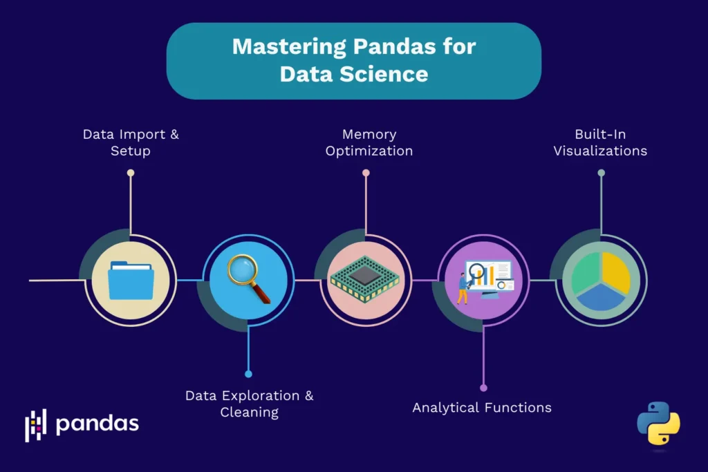
First, we need to bring our dataset into an environment where we can work with it effectively. We’ll use Python, along with the Pandas library, known for its robust data manipulation capabilities. For a comprehensive guide on utilizing Pandas for data science projects, I highly recommend checking out this detailed tutorial: Pandas Complete Tutorial for Data Science in 2022.

Curious about data manipulation with Pandas?
Check out my Complete Pandas Tutorial for practical insights and hands-on examples that make working with data easier, faster, and more efficient.

Now, let’s dive into how you can load the dataset:

import pandas as pd

# Replace '/content/IMDB Dataset.csv' with the actual path to the dataset
df = pd.read_csv('/content/IMDB Dataset.csv')

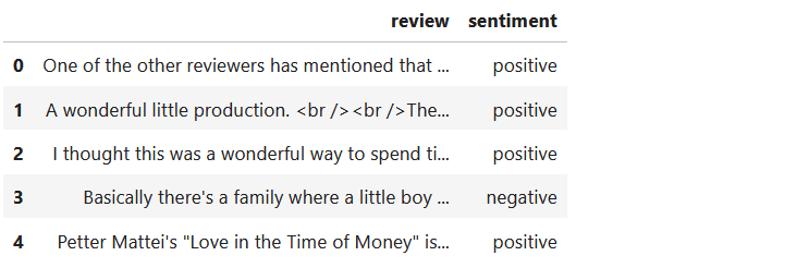
# Disply first 5 rows
df.head()

# Dataframe info
df.info()

This simple code snippet reads the dataset and stores it in a DataFrame df, making it accessible for our upcoming tasks.

Step 2 — Exploring the Dataset

With our dataset loaded, let’s dive into some exploration to understand its structure and content better. This exploration will provide us with valuable insights that are crucial for the next steps.

Checking Sentiment Balance

Ensuring our dataset has an equal number of positive and negative reviews is crucial for unbiased model training:

# Checking Sentiment counts
sentiment_counts = df['sentiment'].value_counts()
print(sentiment_counts)

import matplotlib.pyplot as plt

# Plotting the sentiment counts
df['sentiment'].value_counts().plot(kind='bar')
plt.title('Distribution of Sentiment in the IMDB Dataset')
plt.xlabel('Sentiment')
plt.ylabel('Number of Reviews')
plt.xticks(rotation=0)
plt.show()

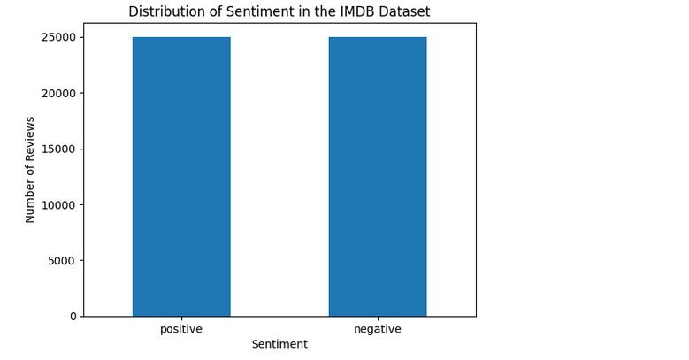
This balance check helps us confirm that our dataset is well-prepared for building a sentiment analysis model.

Review Lengths

Understanding the length of the reviews gives us an idea of the dataset’s complexity:

review_lengths = df['review'].apply(len)
average_length = review_lengths.mean()
print(f"The average review length is: {average_length} characters")

# Plotting the distribution of review lengths
plt.hist(review_lengths, bins=50, color='blue', alpha=0.7)
plt.title('Distribution of Review Lengths')
plt.xlabel('Length of Reviews')
plt.ylabel('Frequency')
plt.show()

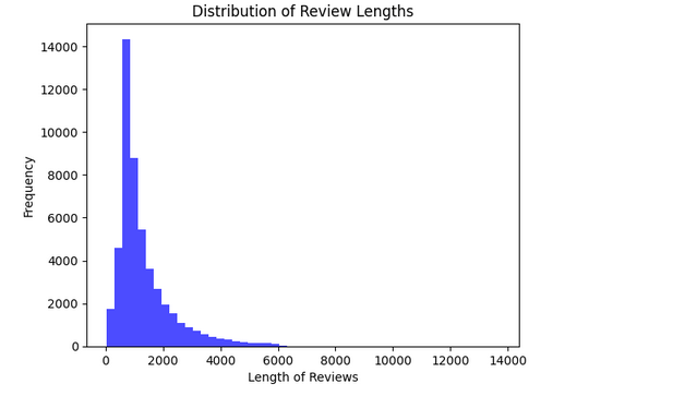
Knowing the average review length assists in preprocessing decisions, such as determining input sizes for our models.

Identifying Common Words

A quick look at the most common words can highlight the dataset’s predominant themes and guide us in refining our text preprocessing:

from collections import Counter
import itertools

words = list(itertools.chain(*df['review'].str.lower().str.split()))
word_counts = Counter(words)

print(word_counts.most_common(10))

import matplotlib.pyplot as plt

# Assuming 'word_counts' is a Counter object of all words
most_common_words = word_counts.most_common(10)

# Unzipping the words and their counts into two lists
words, counts = zip(*most_common_words)

# Creating the bar chart
plt.figure(figsize=(6, 4))
plt.bar(words, counts, color='blue')
plt.xlabel('Words')
plt.ylabel('Frequency')
plt.title('Top 10 Most Common Words in the IMDB Movie Reviews Dataset')
plt.xticks(rotation=45)
plt.show()

While this list will initially include common stopwords, it sets the stage for more targeted text cleaning and preprocessing.

3. Text Preprocessing Techniques

Before we can analyze text data for sentiment or any NLP task, we need to clean and prepare it. This process, called text preprocessing, helps in removing the noise and simplifies the text to a format that’s easier for models to understand.

3.1 The Importance of Text Preprocessing

Text data is often messy and unstructured. It can contain slang, typos, emojis, and varied punctuation. Without preprocessing, these inconsistencies can mislead or confuse your model, leading to inaccurate analyses. Preprocessing standardizes the text, helping models extract meaningful insights more effectively.

3.2. Practical Exercise: Comprehensive Guide to Text Preprocessing

Step 1: Cleaning text

• Removing HTML Tags: Text data, especially from online sources, may contain HTML tags. These tags are useful for web browsers but unnecessary for text analysis and can clutter your data. A regular expression (regex) search-and-replace function is used to identify and remove HTML tags from the text.

import re

def remove_html_tags(text):
    return re.sub('<.*?>', '', text)

# Applying the function to each review in the DataFrame
df['review_no_html'] = df['review'].apply(remove_html_tags)

# Printing both texts
print("Original Text:", df.head(2)['review'].values[1][:100])
print("Processed Text:", df.head(2)['review_no_html'].values[1][:100])

• Lowercasing: Text data often contains words in varied cases. Since “Apple,” “APPLE,” and “apple” would be treated as different tokens by a computer, converting all text to lowercase ensures uniformity and prevents duplication based on case differences. A simple transformation of each token to its lowercase form ensures case consistency across all text.

df['review_lower'] = df['review_no_html'].str.lower()

# Printing both texts
print("Original Text:", df.head(2)['review_no_html'].values[1][:100])
print("Processed Text:", df.head(2)['review_lower'].values[1][:100])

• Removing Punctuation: Punctuation marks, while crucial for grammatical structure, often do not contribute to the semantic meaning of text in analysis and can be removed to simplify the data. Similar to HTML tag removal, a search-and-replace function can strip punctuation from the text, often by using a regex pattern or a predefined translation table.

df['review_no_punct'] = df['review_lower'].str.replace('[^\w\s]', '', regex=True)

# Printing both texts
print("Original Text:", df.head(1)['review'].values[0][:100])
print("Processed Text:", df.head(1)['review_no_punct'].values[0][:100])

While we’ve covered some fundamental preprocessing steps, it’s worth noting that the scope of text cleaning can extend further based on your specific text data and analysis goals. Depending on the nature of your dataset and what you’re trying to achieve with your NLP project, you may also consider:

• Filtering Out Unwanted Words: Certain texts may contain slang, offensive language, or simply irrelevant words that do not contribute meaningfully to your analysis. Identifying and removing these words can help maintain the focus and relevance of your analysis.
• Dealing with Emojis and Special Characters: In today’s digital communication, emojis and special characters are pervasive and can carry significant emotional weight or meaning. Depending on your project’s requirements, you might choose to either remove these elements to simplify the text or analyze them separately to enrich your understanding of the sentiment expressed in the data.

Step 2: Tokenization

What is a Token?

In the world of Natural Language Processing (NLP), a token is the basic building block of text. Think of it as a piece of a puzzle; each token represents a word, phrase, number, or symbol that carries meaning within the context of a sentence or document.

For example, in the sentence “Tokenization simplifies text analysis,” each word, including “Tokenization,” “simplifies,” “text,” and “analysis,” serves as a separate token.

Why Tokenization?

Tokenization serves a critical role in NLP by breaking down complex text into manageable, analyzable pieces. This process:

• Facilitates Text Analysis: By dividing text into tokens, we can analyze and understand the role and meaning of each word or symbol in context.
• Enables Further Processing: Tasks like part-of-speech tagging, sentiment analysis, or named entity recognition rely on tokenized text to function correctly.
• Improves Model Performance: Machine learning models work with numbers, not text. Tokenization is a step towards converting text into numerical data, which models can interpret and learn from.

Implement Tokenization

Implementing tokenization is straightforward with NLP libraries such as NLTK or spaCy. Here’s a simple example using NLTK to tokenize text into words:

import nltk
from nltk.tokenize import word_tokenize

# Ensure you've downloaded the necessary NLTK data
nltk.download('punkt')

# Assuming 'review' is the column with text data we want to tokenize
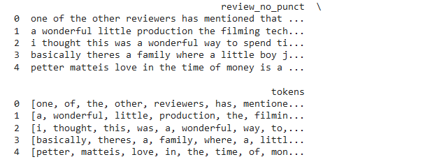
df['tokens'] = df['review_no_punct'].apply(word_tokenize)

# Display the first few rows to verify the tokenization
print(df[['review_no_punct', 'tokens']].head(5))

Step 3: Removing Stopwords

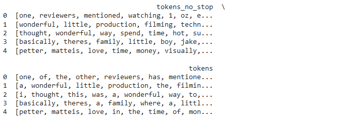
Stopwords are common words (such as “the,” “is,” “in”) that appear frequently in the text but carry minimal semantic value. Removing them helps focus the analysis on more meaningful words. Using a predefined list of stopwords (available in libraries like NLTK), tokens are filtered to exclude any stopwords.

from nltk.corpus import stopwords

# Download necessary NLTK data
nltk.download('stopwords')  # For stopwords

# looking stepwords
english_stopwords = stopwords.words('english')
", ".join(english_stopwords)

stop_words = set(stopwords.words('english'))

def remove_stopwords(tokens):
    return [token for token in tokens if token not in stop_words]

df['tokens_no_stop'] = df['tokens'].apply(remove_stopwords)

# Display the first few rows to verify the after stop word removal
print(df[['tokens_no_stop', 'tokens']].head())

Step 4: Normalization

Normalization in text preprocessing serves to reduce words to their base or root forms. This process helps in treating different variations of a word as the same item, essential for analyzing textual data effectively. There are two primary methods for normalization: Stemming and Lemmatization.

Stemming

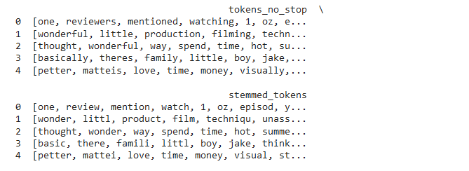
Stemming simplifies words by cutting off the ends, aiming to reduce them to their root forms. This method works on a rule-based process that strips suffixes, which can sometimes lead to incorrect stemming, producing words that are not lexically correct. Despite this, stemming is a fast and resource-light approach to normalization, making it suitable for large datasets where precision is less critical.

Example using NLTK’s PorterStemmer:

First, ensure NLTK is installed and import the necessary components: Next, initialize the Porter Stemmer and define a function to apply stemming to a list of tokens. Then, use the .apply() method to apply this function across our DataFrame’s tokens_no_stop column:

from nltk.stem import PorterStemmer
stemmer = PorterStemmer()
nltk.download('punkt')

# Initialize the Porter Stemmer
stemmer = PorterStemmer()

# Function to apply stemming to a list of tokens
def stem_tokens(token_list):
    return [stemmer.stem(token) for token in token_list]

# Apply stemming to each row in 'tokens_no_stop' and create a new column for stemmed tokens
df['stemmed_tokens'] = df['tokens_no_stop'].apply(stem_tokens)

# Verify the application of stemming
print(df[['tokens_no_stop', 'stemmed_tokens']].head())from nltk.stem import PorterStemmer

Lemmatization

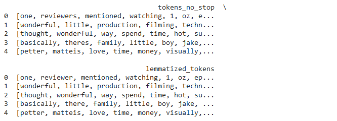
Lemmatization differs from stemming by undertaking a morphological examination of words. This process identifies a word’s lemma, necessitating comprehensive dictionaries for the algorithm to reference and connect the word form to its base lemma. As a result of its thorough analysis, lemmatization achieves greater precision in deriving word roots, ensuring that the produced words are valid in the language.

Let’s Implement Lemmatization, on Our Dataset

First, ensure you have the necessary NLTK library installed and import the components needed for lemmatization:

import nltk
nltk.download('wordnet')

To apply lemmatization, initialize the <strong>WordNetLemmatizer</strong> and define a function that processes a list of tokens. Then, apply this function to the appropriate column in your DataFrame, creating a new column to store the lemmatized tokens:

from nltk.stem import WordNetLemmatizer

# Initialize the WordNetLemmatizer
lemmatizer = WordNetLemmatizer()

# Simple function to lemmatize a list of tokens
def simple_lemmatize(tokens):
    return [lemmatizer.lemmatize(token) for token in tokens]

# Assuming your DataFrame has a column 'tokens_no_stop' containing lists of tokenized words
df['lemmatized_tokens'] = df['tokens_no_stop'].apply(simple_lemmatize)

# Display the first few rows to check the lemmatization results
print(df[['tokens_no_stop', 'lemmatized_tokens']].head())

Applying One Approach

In practice, whether stemming or lemmatization is more useful depends on the specific requirements of your NLP task. Stemming might be your choice for tasks where speed and computational efficiency are paramount. On the other hand, Lemmatization is preferable when accuracy in the representation of linguistic forms is critical, such as in tasks that involve semantic understanding.

It’s essential to choose one method based on your project’s needs, as applying both would be redundant and could introduce unnecessary complexity. Experiment with both techniques and decide which one aligns better with your objectives, keeping in mind that lemmatization generally provides more lexically accurate results but at the cost of higher computational resources.

Bringing It All Together: The Complete Text Preprocessing Pipeline

After exploring the individual components of text preprocessing, we now arrive at the crucial juncture where we consolidate these steps into a single, streamlined process. This comprehensive approach ensures that our text data is meticulously cleaned, standardized, and prepared for any NLP task ahead. Let’s dive into the final preprocessing code that encapsulates our journey from raw text to refined data:

import re
import nltk
from nltk.corpus import stopwords
from nltk.tokenize import word_tokenize
from nltk.stem import PorterStemmer

# Ensure all necessary NLTK data is downloaded
nltk.download('punkt')
nltk.download('stopwords')

# Initialize the essential Porter Stemmer
stemmer = PorterStemmer()

def complete_text_preprocessing(text):
    # Step 1: Remove HTML tags to clean web-scraped text
    text_no_html = re.sub('<.*?>', '', text)

    # Step 2: Lowercase all text for uniformity
    text_lower = text_no_html.lower()

    # Step 3: Eliminate punctuation marks, focusing solely on alphabetic characters
    text_no_punct = re.sub(r'[^\w\s]', '', text_lower)

    # Step 4: Tokenize the text, breaking it into individual words
    tokens = word_tokenize(text_no_punct)

    # Step 5: Filter out stopwords to retain only meaningful words
    stop_words = set(stopwords.words('english'))
    tokens_no_stop = [word for word in tokens if word not in stop_words]

    # Step 6: Apply stemming to reduce words to their root forms
    stemmed_tokens = [stemmer.stem(word) for word in tokens_no_stop]

    # Final Step: Reassemble the processed tokens back into a cohesive string
    cleaned_text = ' '.join(stemmed_tokens)

    return cleaned_text

# Application Example: Preprocess a column of text data in a DataFrame
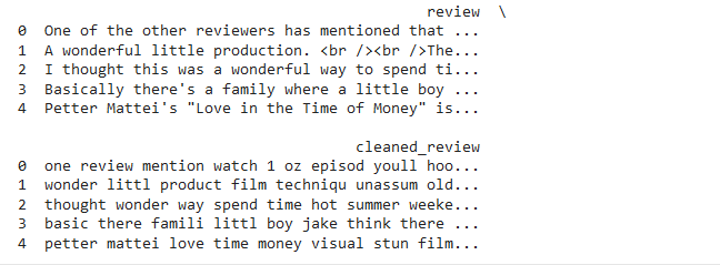
df['cleaned_review'] = df['review'].apply(complete_text_preprocessing)

# Display a preview to verify the transformation
print(df[['review', 'cleaned_review']].head())

Step 5: Vectorization Techniques in NLP

Vectorization in Natural Language Processing (NLP) is a crucial step that translates text data into a numerical format, making it understandable and analyzable by machine learning algorithms. This process is essential for tasks like classification, sentiment analysis, and topic modeling. Two popular vectorization techniques are Bag of Words (BoW) and Term Frequency-Inverse Document Frequency (TF-IDF).

Bag of Words (BoW)

The Bag of Words (BoW) model, a cornerstone technique in natural language processing (NLP), converts text into numerical form by tallying how often each word shows up. It treats the text as if it were a collection of words mixed in a bag, counting their occurrences without regard to the sequence or contextual relationships between them. This simplicity makes it useful across a range of tasks, although its disregard for word order and context may sometimes result in a loss of meaning.

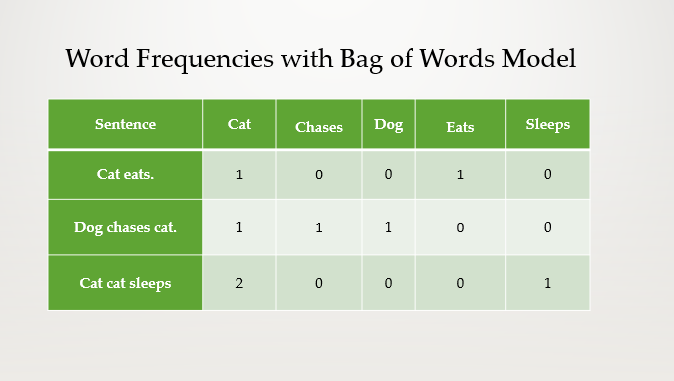
Example: Consider three simple sentences:

• Cat eats.
• Dog chases cat.
• Cat cat sleeps.

The BoW model creates a “bag” that includes all unique words from these sentences. It then counts the occurrences of each word in every sentence, producing a numerical representation:

The Bag of Words model offers a straightforward way to turn text into numbers that machine learning models can work with, making it a cornerstone of text preprocessing in NLP. Despite its simplicity, BoW can be incredibly powerful for tasks where the presence of specific words significantly impacts the analysis, such as text classification and spam detection.

Let’s Implement Bag of Word(BOW) , on Our Dataset

Before coding the Bag of Words model, grasping the max_features parameter is crucial. It limits the vocabulary to the top most frequent words, such as the highest 2000, optimizing computational efficiency and potentially enhancing model accuracy by focusing on the most pertinent words. The best practice for setting max_features involves balancing resource management with the need to capture sufficient textual nuances for your analysis.

from sklearn.feature_extraction.text import CountVectorizer

# Assuming 'df' is your DataFrame and 'cleaned_review' is the column with preprocessed text
bow_vectorizer = CountVectorizer(max_features=2000)

# Apply the vectorizer to the 'cleaned_review' column
X_bow = bow_vectorizer.fit_transform(df['cleaned_review'])

# # Convert the BoW matrix to a DataFrame for better readability
# df_bow = pd.DataFrame(X_bow.toarray(), columns=bow_vectorizer.get_feature_names_out())

# Display the first few rows of the BoW representation
X_bow

TF-IDF (Term Frequency-Inverse Document Frequency)

TF-IDF stands for Term Frequency-Inverse Document Frequency. It’s a technique used to quantify the importance of a word in a document relative to a collection of documents, known as a corpus. The intuition behind TF-IDF is that words that appear frequently in one document but not in many documents across the corpus likely have more relevance to the specific topic of that document.

TF-IDF Calculation

Formula:

Term Frequency (TF)

Term Frequency (TF) is defined as the number of times a word appears in a document divided by the total number of words in that document. It measures the frequency of a term in a document.

Inverse Document Frequency (IDF)

Inverse Document Frequency (IDF) is calculated by taking the logarithm of the number of documents in the corpus divided by the number of documents that contain the word. This metric measures a term’s importance within the corpus.

TF-IDF

TF-IDF is then calculated by multiplying the TF and IDF values together for each term in the document. The higher the TF-IDF value, the more unique the word is to the specific document.

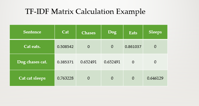
This table now directly correlates the calculated TF-IDF scores with the corresponding sentences from which they were derived, giving a clearer picture of the importance of each word within the context of its document and the corpus as a whole. ​

4. Machine Learning for Sentiment Analysis

With our text data already refined and prepared, we’re set to tackle the essence of sentiment analysis through machine learning. This next phase bridges the gap between raw data and actionable insights, guiding us through the meticulous steps of model training and evaluation. Skipping past further preprocessing, we directly embark on leveraging machine learning techniques to analyze sentiment. Here’s the path we’ll take:

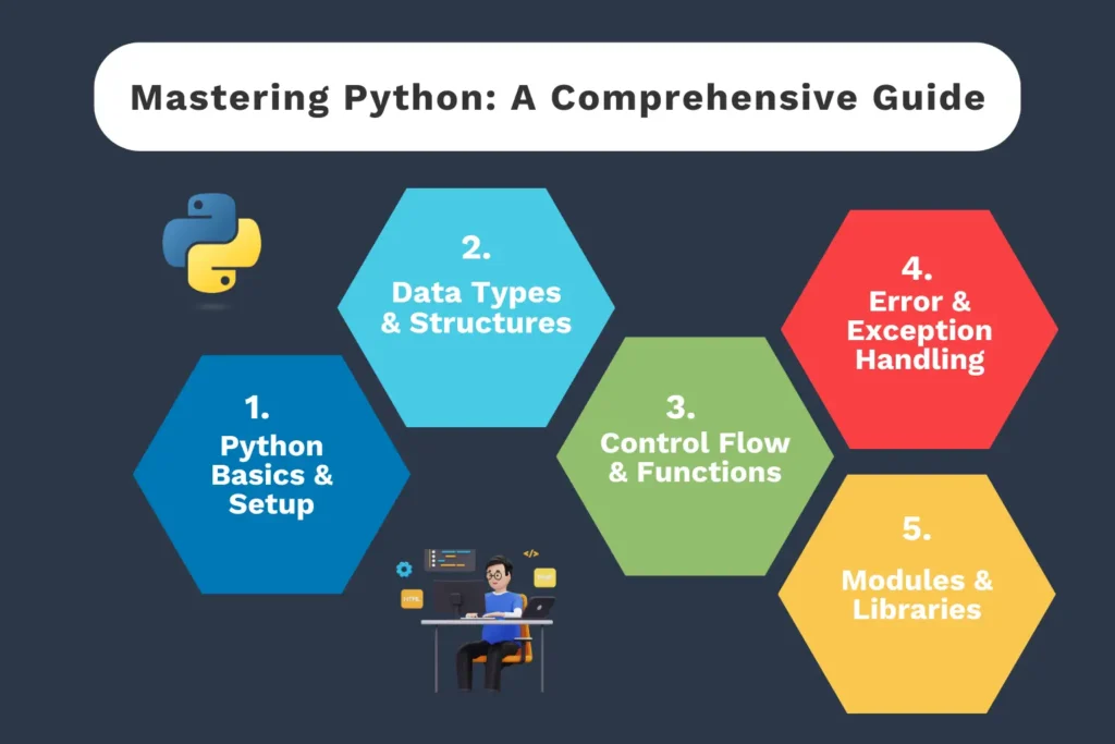
Want to explore more about Python?
Dive into my Comprehensive Python Guide to learn everything from the basics to advanced concepts, designed to help you build a strong foundation and master this essential programming language.

4.1 Practical Exercise: Comprehensive Guide to Machine Learning for Sentiment Analysis

Step 1: Encode Sentiment Labels to Numerical Format

Machine learning models require numerical data to operate efficiently. Hence, we start by converting our textual sentiment labels (such as “positive”, “negative”) into a numerical format.

from sklearn.preprocessing import LabelEncoder

label_encoder = LabelEncoder()
encoded_labels = label_encoder.fit_transform(df['sentiment'])

This step ensures our model can understand the sentiment labels associated with each text entry.

Step 2: Split the Dataset into Training and Test Sets

To evaluate our model’s performance accurately, we divide our dataset into two parts: one for training the model and another for testing its predictions.

from sklearn.model_selection import train_test_split

X_train, X_test, y_train, y_test = train_test_split(
    df['cleaned_review'],
    encoded_labels,
    test_size=0.2,
    random_state=42
)

This split allows us to train our model on a subset of the data and then test it on unseen data, providing an unbiased assessment of its predictive accuracy.

Step 3: Create a Pipeline with TF-IDF Vectorizer and Logistic Regression

A pipeline in scikit-learn helps streamline the process of transforming data and applying a machine learning model. Here, we use the TF-IDF Vectorizer to convert text into a format the model can work with, followed by Logistic Regression for classification.

from sklearn.feature_extraction.text import TfidfVectorizer
from sklearn.linear_model import LogisticRegression
from sklearn.pipeline import Pipeline

pipeline = Pipeline([
    ('tfidf', TfidfVectorizer(max_features=2000)),
    ('clf', LogisticRegression())
])

Step 4: Fit the Model to the Training Data

With our pipeline set up, the next step is to train the model on our dataset.

pipeline.fit(X_train, y_train)

This process involves learning from the training data and adjusting the model to accurately predict sentiment labels.

Step 5: Evaluate Model Performance on the Test Set

Finally, we assess how well our model performs by predicting sentiments on the test set and comparing these predictions to the actual labels.

from sklearn.metrics import accuracy_score
from sklearn.metrics import classification_report

y_pred = pipeline.predict(X_test)
accuracy = accuracy_score(y_test, y_pred)
print(f"Accuracy: {accuracy}\n")
print(classification_report(y_test, y_pred, target_names=label_encoder.classes_))

This step provides valuable insights into the model’s accuracy, precision, recall, and F1-score, helping us understand its strengths and areas for improvement.

Confusion Matrix Visualization

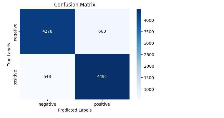
The confusion matrix is a helpful tool for understanding the performance of a classification model. It shows the true labels vs. the predicted labels, allowing us to see the correct and incorrect predictions.

import matplotlib.pyplot as plt
import seaborn as sns
from sklearn.metrics import confusion_matrix

# Generate the confusion matrix
cm = confusion_matrix(y_test, y_pred)

# Plotting the confusion matrix
plt.figure(figsize=(6, 4))
sns.heatmap(cm, annot=True, fmt='d', cmap='Blues', xticklabels=label_encoder.classes_, yticklabels=label_encoder.classes_)
plt.title('Confusion Matrix')
plt.xlabel('Predicted Labels')
plt.ylabel('True Labels')
plt.show()

ROC Curve Visualization

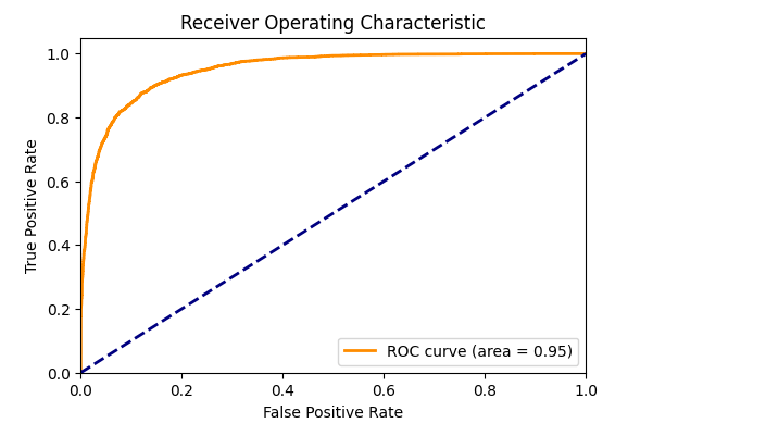
For binary classification problems, the Receiver Operating Characteristic (ROC) curve is a useful tool to evaluate the performance of a model. It plots the true positive rate against the false positive rate at various threshold settings.

from sklearn.metrics import roc_curve, auc
from sklearn.preprocessing import label_binarize

# Binarize the output labels for ROC curve visualization
y_test_binarized = label_binarize(y_test, classes=[0, 1])
y_pred_proba = pipeline.predict_proba(X_test)[:, 1]  # get the probability of the positive class

# Calculate ROC curve
fpr, tpr, thresholds = roc_curve(y_test_binarized, y_pred_proba)
roc_auc = auc(fpr, tpr)

# Plot ROC curve
plt.figure(figsize=(6, 4))
plt.plot(fpr, tpr, color='darkorange', lw=2, label='ROC curve (area = %0.2f)' % roc_auc)
plt.plot([0, 1], [0, 1], color='navy', lw=2, linestyle='--')
plt.xlim([0.0, 1.0])
plt.ylim([0.0, 1.05])
plt.xlabel('False Positive Rate')
plt.ylabel('True Positive Rate')
plt.title('Receiver Operating Characteristic')
plt.legend(loc="lower right")
plt.show()

Note: ROC curve visualization is applicable for binary classification tasks. If your sentiment analysis task involves more than two classes (e.g., positive, negative, neutral), you might focus on the confusion matrix or consider other multiclass evaluation metrics and visualizations.

Step 6: Testing the Sentiment Analysis Model with User Input

After training our sentiment analysis model, it’s essential to evaluate how it performs on new, unseen text. This interactive segment of the code allows you to test the model’s predictions by entering your text. Here’s how you can do it:

while True:
    # Request user input for text analysis
    sample_text_input = input("\nEnter your sample text for sentiment prediction or type 'quit' to exit: ")

    # Exit the loop if the user types 'quit'
    if sample_text_input.lower() == 'quit':
        print("Exiting sentiment prediction tool.")
        break

    # Encapsulate the input text in a list for processing
    sample_text = [sample_text_input]

    # Use the model to predict the sentiment of the input text
    predicted_label_num = pipeline.predict(sample_text)

    # Obtain the probability scores for each sentiment class
    predicted_probs = pipeline.predict_proba(sample_text)

    # Decode the numerical label back to a human-readable category
    predicted_label = label_encoder.inverse_transform(predicted_label_num)

    # Display the predicted sentiment and the confidence level for each class
    print(f"Predicted sentiment: {predicted_label[0]}")
    print(f"Probability scores: {dict(zip(label_encoder.classes_, predicted_probs[0]))}")

This code segment demonstrates the practical application of your sentiment analysis model, offering an immediate way to see how well the model understands and classifies various sentiments expressed in text.

5. Conclusion: Unlocking Insights Through Sentiment Analysis

Congratulations! You’ve successfully navigated through text data preparation, dived into machine learning, and come out with a functioning sentiment analysis model. This journey has equipped you with essential tools for uncovering sentiments embedded within text.

5.1 Key Takeaways

• Foundation: We started with the basics of NLP, focusing on how text preprocessing readies data for analysis, setting a solid foundation for machine learning applications.
• Machine Learning Application: We then shifted our focus to employing machine learning, specifically using Logistic Regression within a TF-IDF framework, for accurately categorizing sentiments.

5.2 Encouraging Further Exploration

The domain of NLP is ever-expanding, filled with new challenges and opportunities:

• Experiment with Different Models: Venture beyond Logistic Regression. Explore models like SVMs, Naive Bayes, and deep learning architectures (RNNs, Transformers).
• Dive into Feature Engineering: Boost your models with various text representation techniques, such as word embeddings or n-grams.
• Hyperparameter Tuning: Fine-tune your model’s settings to achieve the perfect balance between accuracy and overfitting.

5.3 Continuing Your NLP Journey

Your path in NLP doesn’t end here:

• Explore Advanced NLP Tasks: Delve into more complex NLP tasks such as Named Entity Recognition (NER), Part-of-Speech (POS) tagging, and Neural Machine Translation (NMT).
• Stay Updated: The NLP field is continually evolving. Keep up with the latest research and breakthroughs to sharpen your expertise.
• Engage with Open Source: Immersing yourself in open-source NLP projects can provide invaluable hands-on experience and insights into real-world applications.

6. Wrapping Up

Have questions or need guidance?
Feel free to connect with me on LinkedIn, or drop me an email—I’m always eager to collaborate and help fellow learners grow.

Loved this article?
Stay updated with more in-depth insights, tutorials, and resources by subscribing to my blog. Your feedback and suggestions mean the world to me—they help refine content and ensure it delivers maximum value.

For a hands-on experience, don’t forget to explore the GitHub repository accompanying this article. It’s packed with code examples and resources to jump-start your sentiment analysis journey.

7. References:

1. Natural Language Processing — Zero to NLP on Jovian: A comprehensive learning path from NLP fundamentals to advanced concepts. Start learning.
2. Preprocessing Steps for Natural Language Processing (NLP) — A Beginner’s Guide on Medium by Maleesha De Silva: Insights on initial text data preparation for NLP. Read more.
3. Text Preprocessing Techniques for NLP on Medium by Aysel Aynadın: A deep dive into essential text preprocessing methods for NLP. Explore here.
4. Transformers for Natural Language Processing by Denis Rothman on Amazon: Explore the impact of transformers in NLP through various applications. Find it on Amazon.
5. Scikit-learn Documentation: Comprehensive guides on machine learning models, including NLP applications. Scikit-learn Docs.
6. Natural Language Toolkit (NLTK) Documentation: Explore a wide range of text processing libraries with NLTK. NLTK Docs.
7. TensorFlow Text and NLP Guide: Extensive resources for deploying deep learning models in NLP. TensorFlow NLP Guide.
8. Deep Learning for NLP Best Practices on arXiv: Current best practices for deep learning in NLP, from model architecture to optimization. Read on arXiv.

Additional Resources

1. Pandas Complete Tutorial for Data Science in 2022 on Towards AI: Comprehensive guidance on using Pandas for data manipulation, covering basic to advanced techniques. Read the guide.
2. Mastering Python: A Comprehensive Guide for Aspiring Data Scientists on Medium: Detailed exploration of Python in data science projects. Explore the article.

Follow me on Medium , Twitter & LinkedIn