

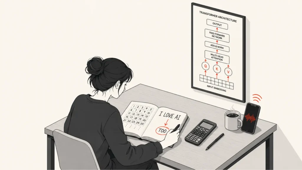
A tiny GPT-style model, small enough to follow by hand, from “I love AI” to the word it picks next
Every large language model you have used, GPT, Claude, Gemini, LLaMA, runs on one idea: the Transformer. Learn how Transformers work and you have learned the shared foundation of all of them. Production language models may contain hundreds of millions to hundreds of billions of parameters and usually have dozens to around one hundred layers. Their vocabularies may contain tens of thousands or even hundreds of thousands of tokens. You cannot realistically follow every calculation with a pencil.
So we shrink it until you can.
Nothing ahead needs more than arithmetic. It does assume you are comfortable with the idea of a model learning patterns from data, so if that part still feels shaky, our guide to machine learning for beginners covers the groundwork first. This article will still be here when you get back.
The clearest way to learn this machinery is to watch it run. So we build a Transformer small enough to follow number by number, then feed it three words:
I love AI
We follow every number, one operation at a time, until the model picks the next word. At each step you get three things: a plain explanation of what is happening and why, a look at how the real models (the original 2017 Transformer, GPT-2, GPT-3, LLaMA) do the same step at scale, and now and then a tip or a question to make it stick.
The numbers are tiny and made up. The machinery is the real thing.
First, a sense of scale
Here is the entire model we will build, next to models that write code and answer questions. They share the same core attention mechanism, but differ in architecture, normalization, positional encoding, and feed-forward design. The GPT-2 figures come from the original GPT-2 paper.
| Model | Embedding dim | Heads | Head dim | Layers | Vocab | Positions | Activation |
|---|---|---|---|---|---|---|---|
| Ours (toy) | 6 | 3 | 2 | 1 | 7 | flat toy values | ReLU |
| Transformer (2017) | 512 | 8 | 64 | 6+6 | ~37K | sinusoidal | ReLU |
| GPT-2 small | 768 | 12 | 64 | 12 | 50,257 | learned | GELU |
| GPT-3 | 12,288 | 96 | 128 | 96 | 50,257 | learned | GELU |
| LLaMA-2 7B | 4,096 | 32 | 128 | 32 | 32,000 | rotary (RoPE) | SwiGLU |
Tip. As you read, keep one eye on the shapes of the matrices. Most confusion in Transformer papers is really just a shape you lost track of. We print the shape after almost every step for exactly this reason.
Our settings in one place:
| Setting | Value | Meaning |
|---|---|---|
| Vocabulary size | 7 | how many words the model knows |
| Input tokens | 3 | length of our sentence |
| Embedding dim | 6 | numbers used to describe each word |
| Heads | 3 | parallel attention “viewpoints” |
| Head dim | 2 | numbers each head works with |
| Blocks | 1 | how many Transformer layers we stack |
Each token is described by six numbers. Attention is split into three heads, so each head works in
dimensions. GPT-2 small makes the same split: 768 dimensions cut into 12 heads gives 64 per head. The arithmetic per head is identical to ours. There is just more of it.
Three family trees, one block
One column in that first table needs explaining before we start building. Why does the 2017 row say 6+6 layers, while every other row says a single number? Because Transformers come in three arrangements, and they are not interchangeable.
| Family | How it reads | Examples | Built for |
|---|---|---|---|
| Encoder-only | the whole sentence at once, in both directions | BERT, RoBERTa | understanding: classification, search, embeddings |
| Decoder-only | left to right, never peeking ahead | GPT, LLaMA, Claude | generation: predict the next token |
| Encoder-decoder | an encoder reads the source, a decoder writes the output while looking back at it | Transformer (2017), T5 | sequence to sequence: translation, summarization |
So 6+6 means six encoder layers followed by six decoder layers. The original paper was a translation model, so it needed both halves. Today’s chat models keep only the second half, which is why every other row in the table carries a single layer count.
We build the decoder-only kind, because that is what powers the models you actually talk to. Everything from Act 2 onward, especially the causal mask, follows from that choice.
Tip. One naming trap worth knowing. The decoder in the 2017 paper has three sub-layers: masked self-attention, then cross-attention that looks back at the encoder, then a feed-forward network. GPT-style decoder-only blocks drop the cross-attention and keep only two: masked self-attention and a feed-forward network. Both get called “the decoder,” but ours is the GPT version, which is why you will not meet a cross-attention step anywhere in this article.
Act 1: Turning words into numbers
A model cannot read letters. It reads numbers. Act 1 is entirely about that conversion.
Step 1 and 2: The vocabulary and token IDs
Think of the vocabulary as the model’s dictionary. We keep it small but relatable, seven everyday words that can form sensible little phrases, so the final prediction actually reads like something a person might say:
| ID | Token |
|---|---|
| 0 | I |
| 1 | love |
| 2 | AI |
| 3 | and |
| 4 | data |
| 5 | math |
| 6 | too |
Our tokenizer maps each word straight to an ID:
From now on the model only sees [0, 1, 2].
In real models: a word may become one token, several subword
tokens, or occasionally part of a token that includes surrounding spaces
or punctuation. Real tokenizers (GPT uses one called BPE) split on
frequent sub-word chunks, so “unbelievable” might become
un, believ, able. Because GPT-2 uses byte-level BPE, it can represent virtually any Unicode string, even when a word was never present as a complete vocabulary token. Our clean one-word-per-ID mapping is the toy version of the same idea.
Step 3: Look up the embeddings
An ID like 2 is just a name tag. It carries no meaning.
So we replace each ID with a small vector of numbers called an
embedding. Picture it as a set of coordinates that
place the word somewhere in “meaning space,” the way latitude and
longitude place a city on a map.
We keep one vector for every word in an embedding table
| ID | Token | Embedding |
|---|---|---|
| 0 | I | |
| 1 | love | |
| 2 | AI | |
| 3 | and | |
| 4 | data | |
| 5 | math | |
| 6 | too |
Looking up [0, 1, 2] just means grabbing rows 0, 1, and
2:
Rows are tokens, columns are features.
In real models: this table is enormous. GPT-2’s embedding
matrix is
Think about it. Our vectors for “I”
Step 4: Add positional encoding
Here is a problem. Attention, which we build in Act 2, compares words to each other but has no built-in sense of order. To it, “Dog bites man” and “Man bites dog” look like the same bag of words. Same words, opposite meaning.
The fix is to stamp each position with its own signature and add it to the embedding, like writing a seat number on every ticket. For readable arithmetic we use flat values:
In real models: the choice of “seat number” is a whole research topic.
- The original 2017 paper used fixed sine and
cosine waves, with one frequency shared by each pair of
dimensions (sine on the even index, cosine on the odd):
- GPT-2 dropped the formula and simply
learned a position table (a
- Many modern decoder-only models, including LLaMA, use Rotary Position Embeddings (RoPE). RoPE rotates components of the Query and Key vectors so their dot products encode relative-position information. Long-context performance still depends on the training context length and the specific RoPE scaling method used.
We use plain
Step 5: Combine into the input matrix X
Now add each position vector to its word’s embedding. Meaning plus place, in one vector:
- I (pos 0):
- love (pos 1):
- AI (pos 2):
This matrix, words fused with positions, is what enters attention.
Act 2: Self-attention, where words start talking
This is the heart of the Transformer, and the part of how Transformers work that most explanations rush, so we go slowly. What follows is self-attention explained one operation at a time. The one-line intuition: every word looks at the other words it is allowed to see, decides how relevant each one is, and pulls in a blend of their information.
The idea behind Query, Key, and Value
Attention borrows the logic of a search engine. Each word produces three vectors:
- Query (Q): what am I looking for? (your search box text)
- Key (K): what do I advertise about myself? (the label on each result)
- Value (V): what do I actually hand over if you pick me? (the content behind the link)
A word’s Query is compared against every word’s Key to score relevance. Those scores become weights, and the weights pull together everyone’s Values. That is attention in one breath.
Each head has its own learned matrices
We run Head 1 in full detail. Then Heads 2 and 3 get the short treatment, because they are the same recipe with different weights, and repeating every multiply would only bore you.
Head 1, step A: the weights and the Q, K, V vectors
Our toy weights simply select two of the six input features for each of Q, K, and V. Head 1 reads features 0 and 1 for its Query, 0 and 2 for its Key, 1 and 3 for its Value:
Multiply
In real models: these are the workhorse weights, learned from data (not hand-picked selectors). GPT-3’s are far larger, but each still just turns a token vector into a Query, a Key, and a Value. Nothing more exotic than the multiply you see here.
Head 1, step B: attention scores Q1 K1 transpose
To score how much one word cares about another, take the dot
product of the first word’s Query with the second word’s Key. A
big dot product means “these two match.” We transpose
Row = the word asking. Column = the word being checked. For instance,
love checking love is
Head 1, step C: scale by square root of d_k
There is a subtle trap. As the head dimension grows, dot products grow with it. Large scores can make softmax excessively sharp and produce very small gradients, making optimization harder. The
paper’s fix is simple: divide by
In real models: identical formula. In the original
Transformer
Think about it. As the head dimension
Head 1, step D: mask the future
We are building a decoder, the GPT family. Its job is to predict the next word, so during training it must never peek ahead. A word may look only at itself and the words before it:
- I can see: I
- love can see: I, love
- AI can see: I, love, AI
Picture sliding a blank card down a page while reading, covering everything ahead. We do this with math by adding a mask that pushes forbidden spots to negative infinity, so they vanish after softmax:
Tip. The causal mask is one of the central differences between GPT-style autoregressive models and BERT-style bidirectional encoders. GPT-style decoders mask the future and predict the next word. BERT uses bidirectional self-attention without a causal future mask (it still uses other masks, such as padding masks) and is trained with masked-token prediction.
Head 1, step E: softmax into attention weights
Now turn raw scores into a clean split of attention. Imagine each word has exactly 100% attention to spend. Softmax decides how to divide it, and every row adds to 1:
Row by row (a lone visible score gets weight 1, and
Read the last row: when predicting after AI, this head splits its attention across all three visible words, leaning most on I.
Head 1, step F: mix the Values
Finally, use those weights to blend the Values,
That is one complete attention head. Every word now carries a little information borrowed from the words it was allowed to see.
Head 2: same recipe, different features
Head 2 repeats every step above, but reads features 2 and 3 for its Query, 1 and 3 for its Key, 0 and 2 for its Value:
Running the same chain (build
Notice the contrast with Head 1. In Head 1, love split its attention almost evenly between “I” and “love.” In Head 2, love leaned mostly on itself (0.703). Same sentence, different focus.
Head 3: the sleepy head
Head 3 reads the newer position-heavy features, 4 and 5 for its Query, 3 and 4 for its Key, 2 and 5 for its Value:
Because this head reads the small positional features, its raw scores
are tiny (the largest is only
Why give a model many heads? Because language has many kinds of relationships at once: grammar (what is the subject?), meaning (what refers to what?), and position (what came just before?). Each head can specialize. Ours already shows the range: Head 1 mixes context, Head 2 focuses sharply, Head 3 stays broad and gentle. GPT-2 small runs 12 heads, GPT-3 175B runs 96, all in parallel.
Act 3: Combining the heads
Step: Concatenate
Each word now holds two numbers from each of the three heads. Glue
them side by side, in order, back to a
Step: Output projection W_o
Gluing is not enough. The three heads worked in separate lanes and
never compared notes. A learned matrix
In real models:
Act 4: Add and Norm, then Feed-Forward
Step: First residual connection (the “Add”)
Here is a small trick with huge consequences. A residual connection just adds the block’s input back onto its output:
- I:
- love:
- AI:
Why add the input back? The residual connection gives both the original representation and the gradient a direct path through the block. Attention adds new context on top of the word rather than replacing it.
Tip. This single “
Step: First layer normalization (the “Norm”)
After all that adding, the numbers can drift to different scales.
LayerNorm rescales each word’s vector on its own to a
steady mean of 0 and variance of 1 (with
Take token I
In real models: the placement of this step evolved. The 2017 paper normalized after the residual add (post-norm). GPT-2 moved it to before each sub-layer (pre-norm) because it trains more stably when deep. LLaMA-style models swap LayerNorm for a lighter cousin called RMSNorm. The goal never changes: keep the numbers well-behaved.
Step: Feed-forward network
Attention let words share information. The feed-forward network (FFN) now lets each word think on its own, with no looking at neighbors. Picture each word stepping into a private booth to process what it just heard:
We use identity weights and zero biases, so the only real action is ReLU, which zeroes out negatives and keeps positives:
- I:
- love:
- AI:
In real models: the FFN is where a surprising share of the
parameters live, because it first expands the
dimension, then shrinks it back. The 2017 paper went
Step: Second residual and second LayerNorm
Add the FFN’s input back (
- I:
- love:
- AI:
Then normalize each word once more. The output of the whole Transformer block is:
Each row is now a context-aware version of its word. Row 1 is “I” after hearing nothing before it, row 2 is “love” after hearing “I,” and row 3 is “AI” after hearing the whole phrase. That is one full decoder block done.
Where are we, big picture? We started with three plain word vectors. We let them talk (attention with three heads), kept the originals safe (residuals), steadied the scale (norm), and let each one reflect privately (feed-forward). Real models repeat this block 12, 48, or 96 times, each one refining the last. We do it once, which is enough to see the whole shape. That single block is the core of how Transformers work, and everything after it is repetition.
Act 5: Predicting the next word
Everything so far has been preparation. This is where we finally see how GPT predicts the next word, by turning one vector into a score for every word the model knows, and those scores into probabilities.
Step: Take the last word’s vector
To predict what comes after AI, we only need the last row. Thanks to the causal mask, it has already soaked up everything before it:
Step: Project into vocabulary scores
Here is the key idea that is easy to miss: at this point, we do not pick a word yet. The model gives a raw score to every word in the vocabulary, all seven of them, and then converts those scores into probabilities. With greedy decoding, the token with the highest score is selected. With sampling, a lower-probability token may also be chosen.
Each score comes from one column of a projection matrix
In our toy every column is only 0s and 1s, which makes each dot
product easy: a
| feature | 0 | 1 | 2 | 3 | 4 | 5 |
|---|---|---|---|---|---|---|
| 1.190 | 0.547 | −0.487 | 1.039 | −0.728 | −1.562 |
Now the total calculation, one line per word (the listed features are
the rows where that word’s column has a
- I selects feature 0:
- love selects feature 1:
- AI selects feature 2:
- and selects features 0 and 1:
- data selects features 3 and 4:
- math selects features 2 and 5:
- too selects features 0 and 3:
Stacking those seven results, in vocabulary order (I, love, AI, and, data, math, too), gives the logits:
We scored all seven words before knowing which would win. The biggest
logit is
Where do the 0s and 1s in
Step: Final softmax into probabilities
One last softmax turns the seven logits into probabilities that add to 1:
| Token | Probability | Percent |
|---|---|---|
| too | 0.4205 | 42.05% |
| and | 0.2571 | 25.71% |
| I | 0.1488 | 14.88% |
| love | 0.0782 | 7.82% |
| data | 0.0618 | 6.18% |
| AI | 0.0278 | 2.78% |
| math | 0.0058 | 0.58% |
The winner is too, and the runner-up and also reads naturally. Our tiny Transformer predicts:
I love AI → too (“I love AI too”)
This time the completion actually makes sense, but do not read too much into that. We chose every weight by hand, so the model has learned nothing; we simply picked a relatable vocabulary and a projection that lands on a sensible word. In a real model, training with gradient descent nudges every embedding and weight until sensible words rise to the top on their own. The machine you just watched uses the same core attention, residual, normalization, and feed-forward ideas found inside GPT. Real GPT models arrange some of these operations differently, most notably by using pre-normalization.
The whole flow on one page
Here is the whole transformer step by step, compressed into one diagram. Every arrow below is something we calculated by hand.
"I love AI"
    |  tokenize
[0, 1, 2]
    |  embedding lookup            (3 x 6)
    |  + positional encoding       X: 3 x 6
    v
Head 1: Q1 K1 V1   Head 2: Q2 K2 V2   Head 3: Q3 K3 V3
    |  QK^T  ->  scale by sqrt(dk)  ->  mask future  ->  softmax  ->  x V
Head 1 (3x2)   Head 2 (3x2)   Head 3 (3x2)
    |  concatenate                 3 x 6
    |  x W_O  (mix the heads)
    |  + residual  ->  LayerNorm
    |  feed-forward (ReLU)
    |  + residual  ->  LayerNorm    Y_final: 3 x 6
    |  take last-word row           h_AI: 1 x 6
    |  x W_vocab                    7 logits
    |  softmax                      7 probabilities
Predicted next word: "too"
Shape cheat-sheet
| Operation | Shape |
|---|---|
| Embedding table | |
| Input after lookup and position, | |
| Per-head | |
| Per-head | |
| Attention scores | |
| Per-head output | |
| Concatenated heads (3 of them) | |
| After output projection | |
| Feed-forward output | |
| Final block output | |
| Last-word vector | |
| Vocabulary projection | |
| Logits and probabilities |
One-line summary of each part
- Embedding: turn a word ID into a vector of features.
- Positional encoding: stamp where each word sits, since attention ignores order.
- Query, Key, Value: what a word seeks, what it advertises, what it hands over.
- Scaling: keep scores from blowing up before softmax.
- Causal mask: stop a word from reading the future.
- Softmax: split a fixed budget of attention into weights that sum to 1.
- Weights times Value: build a weighted blend of information.
- Multiple heads: learn several kinds of relationships in parallel.
- Concatenate plus
- Residual connection: keep the original signal, add the new.
- LayerNorm: keep the numbers stable and comparable.
- Feed-forward: let each word process on its own.
- Vocabulary projection plus softmax: score every possible next word, then turn scores into probabilities.
The one equation to remember
Strip away the scaffolding and the entire attention mechanism is this:
Read it left to right: compare Query with Key,
scale the scores, block the future
with mask
The takeaway
A Transformer does not store human meanings like “love is an emotion.” It stores numbers. Through repeated multiplication, attention, and a few nonlinear steps, refined by training, those numbers come to encode patterns that behave like understanding.
The whole forward pass fits in one sentence:
Turn words into vectors, let every allowed word examine the others, gather the useful information, transform it, and turn the final vector into probabilities for the next word.
You have now seen how Transformers work at the level of individual numbers. We walked through all of it, one calculation at a time, for I love AI, and out came too, creating the phrase I love AI too. Scale this system to billions of parameters and train it on vast amounts of text, and you get models that write code and hold conversations. The same core Transformer math remains, combined with architectural, optimization, and training improvements.
Transformers are one idea among several that make modern AI work. If you want the map rather than the machinery, our guide to AI fundamentals places this architecture next to the other pieces.
Want to go deeper?
If you want to push further into how Transformers work, three places are worth your time, in the order I would take them.
The paper itself. Attention Is All You Need (Vaswani and colleagues, 2017) is shorter and more readable than most people expect. Having just worked through the arithmetic by hand, you will recognise almost every equation in it.
The visual version. Jay Alammar’s The Illustrated Transformer explains the same architecture with pictures instead of numbers. If any step here felt abstract, seeing it drawn often finishes the job.
Build a real one. Andrej Karpathy’s nanoGPT is a working GPT in a few hundred lines of readable code. Everything you followed here, from embeddings and heads to masks, residuals and LayerNorm, is in there doing it for real.